As you start working on STEM project you’ll quickly run into the scenario where you want one device (ie an ESP32 microcontroller) to send data and receive commands from another device (ie a Raspberry Pi or your phone). A simple way to do this is with a MQTT-Node-Red server running on a RPi. You can also add a database (ie Influxdb) to save data for charting in Node-red or Grafana. Data analysis involves measuring, transferring, visualizing, and analyzing the data. Below are tools that I have tried out. There are obviously many more options (ie google data studio) these are just the tools I’ve found easy to learn and useful.

MQTT - Sends data/commands between devices (remote machines and a server)
Influxdb(sql) - Store the data in a time based database
NodeRed(javascript) - Receives the data from mqtt and stores it to the influxdb. Has a gui dashboard with gauges or you can retrieve historical data and chart it. Javascript functions can be written to handle the data flow.

MQTT

Mosquitto MQTT is a lightweight messaging protocol that simplifies sending/receiving messages between devices (messages can be in the form of JSON objects). It acts as a broker to handle mqtt traffic among your devices. The messages are organized by topics. By publishing and subscribing to topics devices are able to talk to each other. For example, you can send commands from a node-red dashboard (web based), via the mqtt broker, to a RPi/esp32 to control servos or motors. And in return the the RPi/esp32 can send status (rpms) or other sensor data (voltage, current, temp) back to the node-red dashboard. The mqtt broker can run on the same RPi involved in the project or on a standalone RPi. The RPi can acts as the mqtt server/broker with node-red as the “brains”. Another example might be collecting the water level of a tank with a sensor and turning a pump off when sensor shows level is high.

Measuring/Sending Data from a esp32/esp8266 or raspberry pi
Data collection can be made through sensors or other instruments

ADC, ina219 current sensor, DHT11 temp sensor, encoder (motor rpm), etc
I then use mosquitto (mqtt) to send the data to a server (usually a raspberry pi) and store it in a database (usually influxdb)

Note - When possible I give each pi a unique name during setup and use hostname.local or just hostname instead of IP address. Using the raw IP address can be problematic due to it changing. Static IP can also be a hassle since you’ll have to make sure your router doesn’t assign that ip address to another machine when it is offline.

Mosquitto documentation can be found at mosquitto.org/man/. It’s a good reference tool for looking at the publish and subscribe functions. (Mosquitto uses port 1883)
Initial setup on the device that will be used as the broker (mqtt server). You will use it both as the broker and client for initial testing.
sudo apt install mosquitto mosquitto-clients
Now run an initial test. Since the subscribe/publish are happening on the broker you do not need to include the broker IP address.
In one window subscribe to “test” topic (-t)
mosquitto_sub -t "test"
In another window publish a msg (-m) to “test”topic (-t)
mosquitto_pub -m "msg from window2" -t "test"
You should see the message show up on the first window

Now add a password file. I called my file “passwd” and put it in /etc/mosquitto
sudo mosquitto_passwd -c /etc/mosquitto/passwd <user>

Password: <enter a password>

Check the status with $ systemctl status mosquitto
The newer version requires a port defined for listening. You can add this in the user config file below sudo nano /etc/mosquitto/conf.d/user.conf

listener 1883

Note - If you look at sudo nano /etc/mosquitto/The mosquitto.conf it states it will also read user config in /etc/mosquitto/conf.d/ directory.

If running the older version of mosquitto it opens port 1883 automatically and will shown in systemctl status mosquitto

To check that port 1883 is listening run sudo lsof -i -P -n | grep LISTEN

You can also tell mosquitto where the password file is by updating the user.conf file
sudo nano /etc/mosquitto/conf.d/user.conf

listener 1883
allow_anonymous false
password_file /etc/mosquitto/passwd

Now test again but this time you’ll have to include your user (-u) and password (-P).
First window
mosquitto_sub -t "test" -u "user" -P "password"
Second window
mosquitto_pub -m "msg from window2" -t "test" -u "user" -P "password"

Enable mosquitto to start on boot
sudo systemctl enable mosquitto

Additional testing -

Default QOS (quality of services) is 0 which has no confirmation that the msg was received. Testing can be done with QOS=1 to get confirmation that the messag was received.
-V to use mqttv311 and -d for debugging
mosquitto_sub -V mqttv311 -t "test" -u "user" -P "password" -q1 -d
Now publish a msg
mosquitto_pub -V mqttv311 -t "test" -m "message" -u "user" -P "password" -q 1 -d

If you have a second device you can try sending a msg from it to the broker. Now you’ll need to specify the IP address of the broker (-h) so mosquitto knows where to send the msg.
mosquitto_pub -h <Broker IPaddress> -m "msg device2" -t "test" -u "user" -P "password"

PAHO Python

RPi mqtt/Python specific libraries - Paho Python client makes it easy to setup the RPi broker functionality. It includes functions for connecting to the broker, sending and receiving messages.
install in venv (.venv)$ python3.7 -m pip install paho-mqtt

Umqttsimple uPython

esp32 mqtt/upython specific libraries - Umqttsimple makes it easy to setup ESP32 communication to the RPi mqtt broker using upython. It also includes functions for connecting to the broker, sending and receiving messages.

On the esp32 you will copy over a umqttsimple.py file along with your boot.py and main.py. You then import it with

from umqttsimple import MQTTClient

The umqttsimple.py code can also be found in github for MQTT projects

Node Red

Node Red is a flow-based coding tool. It has a web browser-based editor where you connect different nodes to retrieve data, store data, make decisions, etc. A common setup is to use the ‘mqtt in’ node to listen for messages/data. Then, based on the mqtt message content (JSON format), other nodes can be connected to store the data in a database, send data to gauges/charts, use a ‘mqtt out’ node to send instructions (publish) to another microcontroller. To program node-red you can use both the built-in nodes or code-blocks with custom javascript code/functions. Using json along with loads/dumps makes it easy to transfer data between Python running on your microcontroller and node-red js.

Although node-red is installed on RPi’s the node-red web site recommends using their script to setup on a RPi.
sudo apt install build-essential git
bash <(curl -sL https://raw.githubusercontent.com/node-red/linux-installers/master/deb/update-nodejs-and-nodered)
On Pi Node-RED works better with the Firefox or Chrome browser
node-red-stop to stop Node-RED
node-red-start to start Node-RED again
node-red-log to view the recent log output
sudo systemctl enable nodered to autostart Node-RED at every boot
sudo systemctl disable nodered to disable autostart on boot

sudo reboot
To setup your node red flows go to http://hostname.local:1880 (IP add = the address of RPi) on any device connected to the network.
For influxdb and gauges/charts options go to menu in upper right and “manage pallette” then install

influxdb
node red dashboard

Dashboard
Once you have gauges/charts setup you can view them at http://hostname.local:1880/ui

Grafana
Most of the graphing I do is in node-red because it’s convenient to setup while working on the main flow and the graphs are compact (look nice on mobile browser). But grafana is useful when you want the ability to zoom in closer and do more analysis. It also has functions to alert you based on conditions you configure.

Installation
Prerequisites
sudo apt-get install -y apt-transport-https
sudo apt-get install -y software-properties-common wget

Add APT key used for authenticating the grafana package
wget -q -O - https://packages.grafana.com/gpg.key | sudo apt-key add - Add the grafana repository to your sources.list echo “deb https://packages.grafana.com/oss/deb stable main” | sudo tee -a /etc/apt/sources.list.d/grafana.list Download package information from the updated sources and install grafana sudo apt update sudo apt install grafana Start the grafana server and enable it to start on boot sudo systemctl start grafana-server sudo systemctl enable grafana-server Grafana runs on port 3000 so you can configure your database by going to http://hostname.local:3000 Initial login is admin/admin. Configuration file is in /etc/grafana/grafana.ini

Add your first data source (influxDB)

InfluxQL
URL: http://localhost:8086
Add a database
Save and Test

Create/add panels in your dashboard

Click on the title and edit (example below)
FROM autogen mydb WHERE device = mcp3008
SELECT field (a0f)
On far right click "Show options" and then Visualation drop down to change graph type to gauge or bar, etc.
Upper right in the referesh bar you can select 5s auto refresh (can't go smaller).

Adding plugin panels (ie plotly) To avoid write permissions I used sudo which forced chown/chmod on the plugin files. There is a better way to do this.. but this is what worked for me. $ sudo grafana-cli plugins install $ sudo chown -R grafana:grafana /var/lib/grafana/plugins $ sudo chmod -R 777 /var/lib/grafana/plugins (could try 742) $ service grafana-server restart Re open grafana and now panels were available

Databases

Influxdb

Some database options

influxdb (time series for monitoring measurements over time)
mysql (relation based) Can be used to collect a set of measurements over varying conditions.
Text, csv, excel file
For time series data I usually use node-red (with its charting options) connected to influxdb
For experimental data I read a csv using Jupyter Notebook or dash plotted by plotly

Influxdb is a time series database (the time stamp is automatically added to the data when storing). It does not require a schema so it is a quick and easy install for collecting data over time. Node-red can store data in the influxdb and retrieve data for charting. (port 8086 used for communication)

Field - used to store the data and is required (not indexed)
Tags - descriptions of the data (metadata). Indexed to make data retrieval faster. Not required but recommended.
Measurement - similar to a table

Note - with ver 1.8+ there is an alternate query option called flux and it differs quite a bit from InfluxQL syntax. The advantage is that flux provides a lot more options for querying and analyzing data. Some examples in my node-red will use flux instead of InfluxQL.

Installation
Add the InfluxDB repository key so the RPi package manager is allowed to search that repository. The key gets passed into the gpg program and de-armored. Then saved into the /usr/share/keyrings/ directory.
curl https://repos.influxdata.com/influxdb.key | gpg --dearmor | sudo tee /usr/share/keyrings/influxdb-archive-keyring.gpg >/dev/null
lsb_release -cs
Add influxDB repository to the sources list using signed-by. lsb_release -cs will automatically fill in the RPi version.
echo "deb [signed-by=/usr/share/keyrings/influxdb-archive-keyring.gpg] https://repos.influxdata.com/debian $(lsb_release -cs) stable" | sudo tee /etc/apt/sources.list.d/influxdb.list

sudo apt update Update the package list. Should see influxdata added
Now install
sudo apt install influxdb
sudo systemctl unmask influxdb.service
sudo systemctl enable influxdb
sudo systemctl start influxdb
journalctl -u influxdb

unmask allows all/any attempts to start the service

For node-red to pull data you need to enable HTTP authentication. With HTTP authentication enabled InfluxDB also requires you to create at least one admin user before you can interact with the system. Enter the influx interface by typing influx at a command line and then create an admin user/pswd.

influx 
CREATE USER admin WITH PASSWORD '<passwd>' WITH ALL PRIVILEGES 
show users 
exit 

Now edit configuration file to enable HTTP authentication.
sudo nano /etc/influxdb/influxdb.conf
Set HTTP service enabled and address

[http] 
enabled = true 
flux-enabled = true 
bind-address = ":8086" 

*Note - After restarting influxdb service you may get “Failed to connect” if trying to enter REPL. It may take 5-15sec to setup and allow you back in.
sudo systemctl restart influxdb
influx -username admin -password <passwd>

Helpful commands

> CREATE DATABASE mydb
(will use default retention policy that equals shard group duration of 7 days. Data will be deleted after 7 days. Shard group is compressed data, stored in a TSM file.)

To use a different retnetion policy ..
> CREATE DATABASE mydb WITH DURATION 26w (default shard for +6mo of data is 1w) 
> CREATE DATABASE mydb WITH DURATION 2w REPLICATION 1 SHARD DURATION 1w 

> DROP DATABASE mydb (to delete) 
> SHOW DATABASES 
> USE mydb 
> SHOW MEASUREMENTS 
> SHOW SERIES 
> SELECT * FROM measurement-name 
> SELECT * FROM temperature 
> SELECT * FROM "temp" WHERE "value" > 0 
> SELECT count(*) FROM temperature; (will show how many recoreds in MEASUREMENT temperature) 

To use influx cli at command prompt
influx -execute 'SHOW DATABASES'

To delete data

>use mydb
> delete from mydb where time > 161798006580600 and time < 161798007032600
> delete from mydb where time = 1617980056650000
> delete from mydb where tag = 'value' 

Retention Policy and Shard. To alter the autogen RP on a db (autogen is the default RP used in nodered influx node)
> use mydb 
> ALTER RETENTION POLICY autogen ON mydb DURATION 2w REPLICATION 1 SHARD DURATION 1w 
> show retention policies 
> show shard groups 

Sharding - facilitates horizontal scaling, or scaling out (vs vertical scaling). Allow for faster processing. Default shard groups based on RP duration.
Retention Policy’s DURATION – Shard Group Duration
< 2 days – 1 hour
>= 2 days and <= 6 months – 1 day
> 6 months – 7 days

CREATE RETENTION POLICY "52weeks" ON "mydb" DURATION 52w REPLICATION 1 DEFAULT

creates an RP called 52weeks that exists in “mydb” database. 52w keeps data for a DURATION of 52w and it’s the DEFAULT RP for the database.
For testing

CREATE RETENTION POLICY "1d" ON "mydb" DURATION 1d REPLICATION 1

will keep data for 1 day. Have 1 day to get the testing data retrieved and saved offline in a spreadsheet.

To export a database/table(measurement) to a csv file
influx -database 'database name' -execute "SELECT * FROM measurement" -format csv > test.csv

To backup/restore data
sudo -u influxdb influxd backup -portable -host <IPadd>:8088 /path/to/backup/
sudo -u influxdb influxd restore -portable -host <IPadd>:8088 /path/to/backup/

To change the location where your data is stored
Create data and meta folders in the newlocation
Make influxdb owner of these new locations
sudo chown -R influxdb:influxdb newlocation/influxdb/meta/
sudo chown -R influxdb:influxdb newlocation/influxdb/data/
Update permission
sudo chmod 777 -R data
sudo chmod 777 -R meta

changed folders in /etc/influxdb/influxdb.conf to /home/pi/influxdb (data and meta) along with IP address and under [http] at bottom enable=true for endpoint and bind-address = 8086

MariaDB

Mariadb is based on mysql. Port 3306

Note for remote connection from excel. Will need to configure mariadab config file by commenting out bind statement and add user privileges to all db and wild card host (see comments below). Also may need to install ODBC (Open DataBase Connectivity) connector from https://dev.mysql.com/downloads/connector/odbc/ and visual studio update. Then search/open up ODBC 64bit administrator and add MySQL ODBC 8.0 ANSI driver. Set up the connection and chose SQL server authentication.

Run sudo apt update to update the package list

sudo apt update
sudo apt install mariadb-server
sudo mysql_secure_installation utility
(options to allow for remote access on port 3306)
*sudo mysql -u root -p
sudo ufw allow mysql
sudo systemctl start mysql
sudo systemctl enable mysql
Config file is at /etc/mysql/mysql.conf.d/mysqld.cnf

If you don’t run as sudo then the first time you get “MySQL ERROR” then run as sudo

$ sudo mysql
Then run alter command at mysql prompt
sql mysql> ALTER USER 'root'@'localhost' IDENTIFIED WITH mysql_native_password BY 'your_new_password';
CTRL-D to exit

Create a db with CREATE DATABASE name;
Then create a user and privileges
CREATE USER 'username'@'localhost' IDENTIFIED BY 'password';

GRANT ALL PRIVILEGES ON <dbname>.* TO 'username'@'localhost';
FLUSH PRIVILEGES;

Can check user login with same sudo mysql -u user -p
To see users
SELECT User, Host FROM mysql.user WHERE Host <> 'localhost';

To grant remote access you wild card all db with * and use % to wild card IP addresses
GRANT ALL PRIVILEGES ON *.* TO 'sj4u'@'192.168.100.%' IDENTIFIED BY 'password' WITH GRANT OPTION;

Firewall config

firewall config  
firewall-cmd --add-port=3306/tcp 
firewall-cmd --permanent --add-port=3306/tcp

Configuration file is in /etc/mysql/mariadb.conf.d/50-server.cnf
for remote access may need to update bind-address from 127.0.0.1 to 0.0.0.0 or comment it out
and add

skip-networking
skip-bind-address

and restart with sudo systemctl restart mysql.service
can see starting param with mysqld --print-defaults

or install PHPMyAdmin
sudo apt install php libapache2-mod-php
sudo apt install phpmyadmin
Select apache web server and say No to config with dbconfig-common

Go to http://RPi-IPAddress/phpmyadmin
if you need to restart the server use sudo service apache2 restart

Test connection with mysql --host=localhost --password='password' --protocol=tcp --port=3306 esp2nred

Common mysql commands

SHOW DATABASES;
USE <database>;
SHOW TABLES;
SELECT * FROM <table>;
UPDATE, INSERT, DELETE```

To import a csv (can also save a xls file as csv)  
Create a database and empty table with fields then import with the LOAD command.  
--local-infile may be needed  
* ```$ mysql -u root -p --local-infile```  
```sql
mysql> CREATE DATABASE testdb;
mysql> USE testdb;

Create the table/define schema using options below
A good example is in node-red

mysql> CREATE TABLE mytable (
'no' INT NULL AUTO_INCREMENT,
'date' TIMESTAMP NOT NULL,
field1 INT NOT NULL PRIMARY KEY,
field2 VARCHAR(20),
field3 DATE,
field3 INT,
field4 FLOAT);

Now import the data with LOAD

mysql> LOAD DATA LOCAL INFILE "/path/to/data.csv" INTO TABLE testdb.mytable FIELDS TERMINATED BY ',' LINES TERMINATED BY '\n' IGNORE 1 LINES (field1, field2, @field3, field4) set field3 = NOW();

Description:
column_name data_type(length) [NOT NULL] [DEFAULT value] [AUTO_INCREMENT] column_constraint;

column_name
data type and optional size VARCHAR(255)
NOT NULL ensures the column will not contain NULL. Other options are CHECK and UNIQUE.
DEFAULT is default value for the column.
AUTO_INCREMENT col is incremented by one automatically whenever new row is inserted. Each table can only have one AUTO_INCREMENT column.
After the column list can define table constraints like UNIQUE, CHECK, PRIMARY KEY and FOREIGN KEY.

To verify

mysql> SELECT * FROM mytable ORDER BY field1;

mysql> SELECT * FROM mytable limit 10;

MS Access

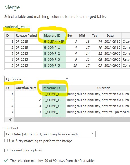
Access makes importing data into excel convenient. You can use PowerQuery to import sheets and transform them. You can also modify tables (add col/rows) with append/merge using the gui and drop down menus vs writing a query.

Basic Charting

For time series data I usually use node-red (with its charting options) connected to influxdb. This is the easiest/quickest setup.

Node-Red Charts/Gauges

Node-red can store/retrieve data from a db like influxdb. Has basic line graphs and charts for monitoring data over time. Options to read/write text files, too

Grafana

Grafana has more advanced charting features. Data from the influxdb can also be accessed thru grafana (geared for time series data)

Advanced Data Visualization

For more advanced data analysis options

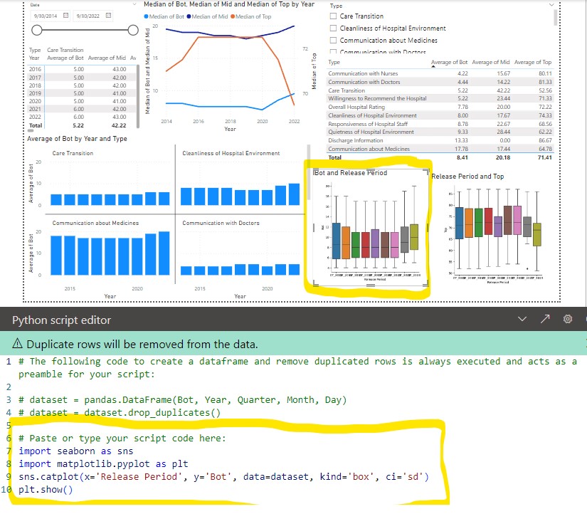
Jupyter notebook with pandas, numpy, matplotlib, seaborn and dash as the interactive portion.
Power BI (microsoft windows based). Can import data from databases, csv, JSON, etc and do basic plotting with microsoft tools. Can add R/Python scripts to do more advanced box plots, histograms, heat maps, etc with plotly.
dash is Python based dashboard using plotly to do advanced box plots, histograms, heat maps.
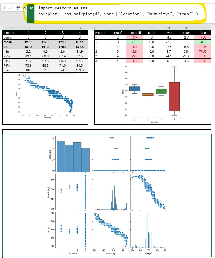
Python in excel allows you to enter python code in an excel formula bar and execute it. You can then output the plot or table into your spreadsheet. An advantage of this is you can leverage off pandas to quickly duplicate/transform data tables without changing the original data. You also have access to the python statistical functions. Also if you already have python/jupyter/dash code for reports you can now copy these into excel (or Power BI).
streamlit is a quick and easy data visualizations.
Pandas

Pandas is a python library (built on top of NumPy) that provides a tabular structure to your data for most of the advanced data visualization tools. Typically one of the first steps you will do is import your data from a database, spreadsheet, or csv into a pandas dataframe. From here you can easily duplicate the dataframe, modify, create pivots, format columns, add data, etc. An advantage of this is you can easily/quickly transform your data without affecting your original database.

 df = pd.DataFrame(client.query_api().query_data_frame('from(bucket: "esp2nred") |> range(start: -5d) |> pivot(rowKey:["_time"], columnKey: ["_field"], valueColumn: "_value")'))
    df = df.drop(columns=['result', 'table', '_start', '_stop', '_measurement', 'device'])
    df = df.assign(date=df['_time'].dt.strftime('%Y-%m-%d'))
    df['date'] = pd.to_datetime(df['date'])

Results = multi.pairwise_tukeyhsd(df['tempf'], df['location'], alpha= 0.05)  # Use multi pairwise tukey HSD
dftukey = pd.DataFrame(data=Results._results_table.data[1:], columns=Results._results_table.data[0])
dftukey['reject'] = dftukey['reject'].astype(str)
table_tukey = dbc.Table.from_dataframe(dftukey, striped=True, bordered=True, hover=True) # use bootstrap formatting on table

# Create summary dataframe with statistics
dfsummary = df.groupby('location')['tempf'].describe()  # describe outputs a dataframe
dfsummary = dfsummary.reset_index()  # this moves the index (locations 1,2,3,4) into a regular column so they show up in the dash table
'''dfsummary.style.format({   # this would work if the values were floats. However they
    "mean": "{:.1f}",         # were strings after the describe functions so had to use
    "std": "{:.1f}",          # the map function below
})'''
dfsummary.loc[:, "mean"] = dfsummary["mean"].map('{:.1f}'.format)  # format as float. see comment above
dfsummary.loc[:, "std"] = dfsummary["std"].map('{:.1f}'.format)
dfsummary.loc[:, "50%"] = dfsummary["50%"].map('{:.1f}'.format)
dfsummary = dfsummary.set_index('location').T.rename_axis('location')
dfsummary = dfsummary.reset_index()
print(dfsummary)
table_summary = dbc.Table.from_dataframe(dfsummary, striped=True, bordered=True, hover=True) # use bootstrap formatting on table

Python In Excel

Python in excel allows you to enter python code in an excel formula bar and execute it. You can then output the plot or table into your spreadsheet. An advantage of this is you can leverage off pandas to quickly duplicate/transform data tables without changing the original data. You also have access to the python statistical functions. Also if you already have python/jupyter code for reports you can now copy these into excel (or Power BI).

Jupyter Notebook

Jupyter Notebook is easily started from anaconda in either windows, mac, or linux. A typical flow

from IPython.display import display 
import pandas as pd
import numpy as np
from matplotlib import pyplot as plt
import seaborn as sns

df = pd.read_csv("data.csv")

pivoted = pd.pivot_table(df, values='data', index=['file', 'sample', 'sensor'], columns = ['type']).reset_index()

pivoted.groupby(['file']).mean().round(1).drop(['sensor', 'ave', 'delta', 'raw'], axis=1)

pivoted.groupby(['file']).describe().round(1).drop(['sensor', 'delta', 'raw', 'ave'], axis=1)

# Use melt to unpivot
comparedf = pd.melt(pivoted, id_vars=['file', 'sample', 'sensor', 'delta', 'time'], var_name='stat')

a = sns.catplot(x='stat', y='value', col='file', data=comparedf, kind='box', ci='sd')
plt.show()

b = sns.catplot(x='stat', y='value', data=comparedf, hue='sensor', col='file', kind='strip')

# More seaborn options
fig,axs = plt.subplots(1,2, sharex=False, sharey=False, squeeze=True)
g = sns.boxplot(x='file', y='time', data=pivoted, ax=axs[0])
#g.set(ylim=(1500, 2250)) g.set_title('ADC Time') g.set_ylabel('time (ms)')
#plt.title('ADC Average')
#plt.ylim(1500, 2250)
#h = sns.boxplot(x='file', y='raw', data=pivoted, ax=axs[1])
#h.set_title('ADC Raw') #plt.title('ADC Raw')
#plt.ylim(1500, 2250)
#h.set(ylim=(1500, 2250))
#h.set_ylabel('raw')
plt.show()

# Histogram

pi0df = pivoted[pivoted['file'] == 'pi0']
esp32df = pivoted[pivoted['file'] == 'esp32']
sns.distplot(pi0df[pi0df['sensor'] == 0].raw, label='pi0-ch0')
sns.distplot(pi0df[pi0df['sensor'] == 1].raw, label='pi0-ch1') sns.distplot(esp32df[esp32df['sensor'] == 0].raw, label='esp32-ch0') sns.distplot(esp32df[esp32df['sensor'] == 1].raw, label='esp32-ch1')
#fig.legend(labels=['pi0-ch0','pi0-ch1','esp32-ch0','exp32-ch1'])
plt.legend()
plt.show()

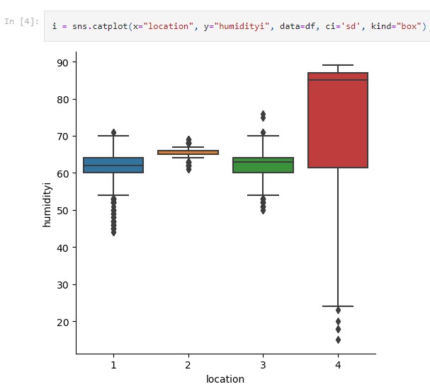
​# Seaborn categorical plot. kind="box"
i = sns.catplot(x="file", y="time", data=pivoted, ci='sd', kind="box")

Dash-plotly

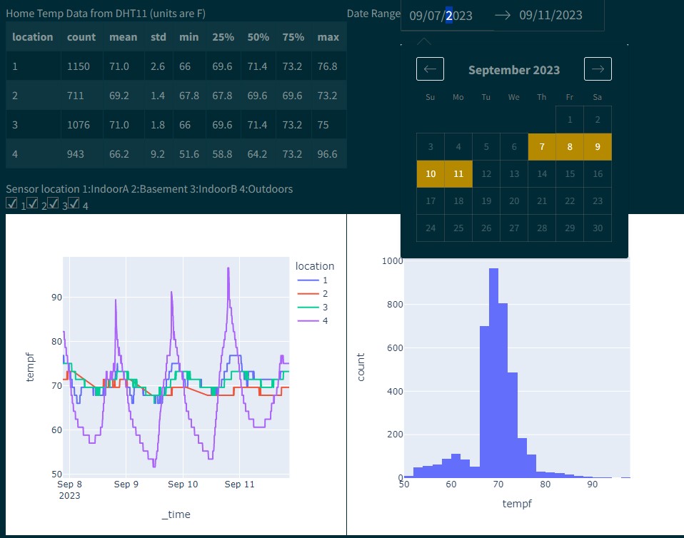
Dash gives more GUI type functions, ie letting a user toggle data series on/off while plotting.
$ python3 -m pip install dash

You will create a file called app.py that contains the dash/plotly code.
When you run
$ python3 app.py
It will create a link to view the charts in your browser

Primary components
(initial chart can be plotted with steps 1-3 alone)

Load css and create dash object
Define figures (charts. ie fig = px.histogram(df, x=”values”, nbins=1 ), optional text string (markdown), functions(ie to show the data/df)
Layout (see below.. will use html and core components)
Callbacks (not required but can be used for interactive charts)

More details

Layout is a hierarchical tree (dash_html_components)
Use html components (classes for HTML tags) to create the layout (ie html.DIV, style, etc).
To place charts use dash_core_components: dcc.Graph(figure=fig)

Callbacks
Callbacks allow for input/output. Makes the charts dynamic and gives you more options for control in the web interface (from dash.dependencies import Input, Output)

@app.callback(Output(output_args), Input(input_args))
def generateChart(x,y):
   fig = px.box(df, x=x, y=y)
   return fig

Packages to import

import dash
import dash_core_components as dcc
import dash_html_components as html
from dash.dependencies import Input, Output
import plotly.express as px
import pandas as pd

Power BI

Power BI (microsoft windows based) is great for clean visualization in a presentation/powerpoint style. It is geared for presenting. It can import data from databases, csv, JSON, etc and do basic plotting with microsoft tools. Can add R/Python scripts to do more advanced box plots, histograms, heat maps, etc with plotly. Only supports importing from pandas (df).

Workflow

This is my general workflow I follow for projects. I often start with RPi/Python and then translate it to esp32/uPython.

For comparing different hardware options (RPi vs esp32) and power supply/memory considerations start at the hardware section.

If setting up a new Raspberry Pi for the project.

Use RPi imager to install the Raspberry Pi OS. (I usually install the full version and then remove programs I do not need.) Click on the options for RPi imager and you can enter setup info like a unique hostname, wifi info, etc. This makes it easier to setup without a monitor.
Plug the RPi and go through the setup screens.
Go to ‘Raspberry Pi Configuration’ Menu and ‘Interfaces’ and turn on SSH/VNC for remote Pi operation (may also need to turn on SPI, I2C, or 1-wire, depending on the hardware you’re connecting). After reboot you can note the IP address and use it with RealVNC viewer to connect remotely from a desktop PC/laptop. (Giving the RPi a unique hostname and using it is useful since the IP address will not stay constant. Or set-up a RealVNC connect account and connect even from a different wi-fi. Free for Raspberry Pi)
To free up space and minimize the time required for updates remove programs that are seldom used. See bottom of my list of software page. Before installing programs/packages it is always a good idea to do an update ($ sudo apt update && sudo apt upgrade)
(optional - to change the RPi appearance/desktop and/or customize the desktop start at RPi options. For details on how installing packages work continue on to software package section)
gdebi is what I use for installing DEB packages ($ sudo apt install gdebi)
VScode is the main editor I use.
Git is what I use for maintaining project code (follow setup of ssh key if you’re going to maintain the code on github).

Hardware

Hardware/Circuits/Sensors/Peripherals - Adafruit libraries are what I primarily use to simplify getting data from sensors (Adafruit also has a line of SBCs and useful parts/circuits for projects). The libraries are primarily written in circuitpython to work with Adafruit SBCs but they also have a Python/RaspberryPi compatability tool called blinka that will install board module. Most projects will use either Raspberry Pi specific GPIO libraries called RPi.GPIO, which are installed on RPis by default, or more generic gpiod C library/tools for working with Linux GPIO hardware. gpiod is the tools, libgpiod2 is the library, python3-libgpiod allows Python to use the library.
sudo apt-get install libgpiod2 python3-libgpiod gpiod

For simple gpio functions like turning an led on/off I will use gpiozero. gpiozero is an interface that simplifies the code for working with the pins. If you’re not working in a virtual environment then gpiozero can use the RPi.GPIO modules, installed on RPi by default, or pigpio modules for the pin factory. However when working in a venv I’ve noticed I have to specifally use pip3 to install RPi.GPIO (or pigpio) in my env for gpiozero to see the modules.

Also when possible check that hardware/circuits work before soldering or trying to control it with software. Some examples

Connect LED to 3.3V and confirm it lights up.
Use a servo tester to confirm the servo motors work.
Use alligator clips to hook up a 18650 battery to a li ion charger and the device it will power. Confirm charging/discharging works. I’ve come across multiple bad chargers. They work fine with no load but would shut off with even .25 Watt load.
The hardware trouble shooting section is good to understand before moving on to more advanced projects.
For I2C make sure tools installed
- sudo apt install -y python-smbus
- sudo apt install -y i2c-tools

Coding

Initialize an empty github repository
Select the option to create the README and .gitignore (python template) github
Copy the ssh link under Code
Clone the empty repository - Cloning can either be done inside an editor like VScode or going to the RPi the project will be done on (often using vnc) and clone the repo with $ git clone git@github.com:user/repo.git (ssh link copied from github). Or inside VScode connect to your github account, remote to the RPi and in the pallette type git clone. Search for the repository and select the location to clone to.
Start Coding - The setup I’ve found myself using most is VScode. I use the VScode remote connection extension to connect to the RPi’s and code from another linux/windows PC. (The exception is Pi0. The VScode remote extension does not work on Pi0. So for Pi0 projects I configure the Pi0 git project folder as a samba share and use a txt editor to work on the code from a PC.)
In VScode remote connect to the RPi3-4
Open the cloned github folder and confirm .gitignore is setup.
Open the terminal and create virtual env. Can install/use other python, ie python3.7
$ python3.7 -m venv .venv
$ source .venv/bin/activate and confirm Python (.venv) interpreter selected in bottom
Install any required packages. ie $ python3.7 -m pip install ‘package’

Get first pass, functional code working on “main” branch
Code, test, code, test, etc

I use the git commit/syncronize to keep the code uploaded to github. This keeps a backup and makes it easier to transfer and test on other devices.
Add functionality by creating a develop branch and merging it back with the main when complete. (see functionality section below)
If using a venv and need the program to run outside of the venv environment (ie need it to run on startup) then make sure to update the shebang #! header of your python file to point to the python path in your venv. Example #!/home/pi/projectA/.venv/bin/python3
You can then make it executable with $ chmod +x filename.py
Now you can run the program with $ ./filename.py

MQTT/Servers/DB

Sending commands, collecting data - Most projects involve remote commands, sending instructions, and collecting data. I use mqtt, node-red, influxdb for this. I have a Pi3B dedicated as a mqtt/node-red server. Login at hostname.local:1880 and create node-red flows. (* I give each Pi a different hostname and use hostname.local instead of IP address when possible. The IP address can be problematic when switching from stand alone to wifi connected)

esp32/uPython

Translate to esp32 - In the git folder create a /upython folder and copy boilerplate/template main.py code for whatever type of project. The esp32 will be connected to USB port. Two options below for coding esp32. Both have pros/cons.

RPi and Thonny - Remote connect from a PC and using Thonny copy code from the upython folder to the esp32. Code, test, code, test, etc. When completed copy the code from esp32 back to git project folder and sync using VScode.
Linux PC and VScode with Pymakr. Can use VScode to edit and sync directly

Run at Startup

There are multiple methods to enable a program to run at startup. For a full list check the autostart/start-on-boot section. If using a virtual env; to statisfy dependencies make sure your python program has a shebang header pointing to the python path in your virtual env. example.

!/home/pi/project_dir/.venv/bin/python3

And make the program executable with sudo chmod +x program.py

A quick systemd setup can look like this
sudo nano /lib/systemd/system/program_name.service

[Unit]
Description=Python Program to Run at Startup

[Service]
User=pi
Group=pi

ExecStart=/home/pi/project_dir/program.py
Restart=on-failure

[Install]
WantedBy=multi-user.target

Call graph A call graph can be helpful to visually see which functions are calling which functions.

Install graphviz $ sudo apt install graphviz or can try linuxbrew
In activated venv install project graph $ python3x -m pip install git+https://github.com/fior-di-latte/project_graph.git
Inside project directory run $ project_graph your-program.py
A .png file should be created.
If a graph.dot is created but no .png then try $ dot -Tpng graph.dot > output.png

Another method is pycallgraph2

Install graphviz $ sudo apt install graphviz or can try linuxbrew
In activated venv install graphviz $ python3x -m pip install pycallgraph2
Inside project directory run $ pycallgraph graphviz – ./mypythonscript.py

Git branches

If you will be adding features use git branches. “main” will be the default primary code. Work on main branch until you have preliminary working code (useful to test initial functions and confirm everything is operating)

Add More Functionality (branch from develop)
To keep your initial main branch in-tact while working on features create a permanent develop branch that you branch off of.

$ git checkout -b develop main (branch off from develop for features)

Now create branches for features

$ git checkout -b feature1 develop (creates feature branch and checks it out)
Can create and work on multiple features and make commits

When finished, merge the feature back into develop branch

$ git checkout develop (switch from feature back to develop)
$ git merge --no-ff feature1 (merge develop and feature1)
$ git branch -d feature1 (delete the feature1 branch)
$ git push origin develop (update the remote repo)

When you’ve completed all features and want to update main

$ git checkout main
$ git merge develop

Bug Fixes (branch from main)

$ git checkout -b hotfix1 main (creates hotfix branch and checks it out)
Can work on the bug and make commits

Merge the bug fix back into main and develop branch

$ git checkout main
$ git merge --no-ff hotfix1
$ git checkout develop
$ git merge --no-ff hotfix1
$ git push origin develop (update the remote repo)
$ git push origin main (update the remote repo)
$ git branch -d hotfix1 (delete the hotfix branch)

Other helpful commands (.venv)$ python3 -m pydoc -n IPaddress (browse thru the installed package/modules)
(IPaddress = 0.0.0.0)
To find files use grep -r 'name' .
To browse pi use
python3 -m http.server

If you have a monitor hooked up to the RPi (or VNC) you can use VScode for a gui alternative to many of the command lines. Will also want to make sure you have a keyring setup with VScode for git functions. nano .gitconfig (confirm your git setup)
Inside VScode ```console F1 Git: Clone Clone from GitHub A list of your repositories will come up. Select the Repository and the folder to clone it in.

Now you can do New Terminal, create/activate .venv and install from requirements.txt

(if using vscode ssh for remote work may need to install python extension after connecting) ```

Copy Project

To transfer project to another system
Output the python packages required to a requirements.txt file
(.venv)$ pip3 freeze > requirements.txt
or $ python3 -m pip3 freeze > requirements.txt

Confirm the git remote and push to github $ git remote -v $ git add . $ git commit -m “message details” $ git push -u origin main (or $ git push)

Go to new device/location $ git clone git@github.com:user/repo.git (ssh copied from github)

Create/activate a .venv $ python3 -m venv .venv $ source .venv/bin/activate install with -r for requirement install (.venv)$pip3 install -r requirements.txt or $ python3 -m pip3 install -r requirements.txt

(if using vscode ssh for remote work may need to install python extension after connecting)

Create Python Package

Python Package - If the code/project will be used in many other projects create it as a package that you can import. This will keep your main code more organized and smaller.

Create a package folder with init.py
init.py - There are multiple approaches to the import
- import package.module
- from .module import classA
Put the module code in the package folder and use name == “main”: to run module as stand alone script.
For the top script use appropriate import based on package init (1:from package import module as xx or 2:import package)
Call the functions (var=xx.function() var = package.classA())

(../../../ref/coding/starting-up/)

Images can you col-# col-sm-# col-md-# col-lg-# Use auto to auto size around image Just wrap your images with <div class="col-sm"> and place them inside <div class="row"> (read more about the Bootstrap Grid system).